Physical Quantities and Measurement Techniques
Measuring Tools
Rulers and measuring cylinders are fundamental instruments for determining length and volume.
- A ruler measures length by reading markings directly, with accuracy limited by tick spacing resolution.
- A measuring cylinder determines liquid volume, requiring careful eye-level alignment with the meniscus to eliminate parallax error.
- Clocks and digital timers measure duration intervals. Reaction delay affects human-timed measurements, making digital timers preferable for short intervals where precision matters.
Pendulums enable accurate time measurement by exploiting oscillation properties.
A single oscillation period is susceptible to reaction errors, so measuring multiple oscillations $n$ and dividing the total time $T_{\text{total}}$ yields the average period.
The formula is $T = \frac{T_{\text{total}}}{n}$, which reduces timing uncertainty proportionally to the square root of the measurement count.
Scalars vs Vectors
Physical quantities are classified by their properties.
-
Scalars
- Possess magnitude but no direction
- Examples: distance, speed, time, mass, energy, and temperature.
-
Vectors
- require both magnitude and direction
- Examples: force, weight, velocity, acceleration, momentum, electric field strength, and gravitational field strength.
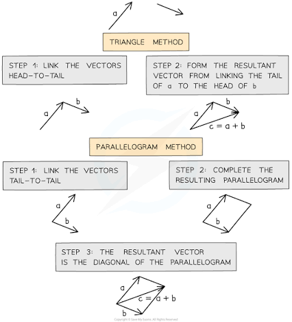
Resultant of Two Vectors
The resultant of two vectors at right angles uses vector addition. The magnitude combines components via Pythagoras theorem:
$R = \sqrt{A^2 + B^2}$
The direction from one component is determined using inverse tangent:
$\theta = \tan^{-1}\left(\frac{A}{B}\right)$
Worked example: Two forces of 30 N and 40 N act perpendicularly.
The resultant magnitude is $R = \sqrt{30^2 + 40^2} = \sqrt{2500} = 50\text{ N}$.
The direction is $\theta = \tan^{-1}\left(\frac{30}{40}\right) = \tan^{-1}(0.75) = 36.9^\circ$.
Motion
Definitions
Speed
- quantifies distance covered per unit time as a scalar value.
- The formula $s = \frac{d}{t}$ calculates speed from distance and time.
Velocity
- extends speed by incorporating direction, making it a vector quantity.
Average speed
- calculates total distance divided by total time,
- defined as $v_{\text{avg}} = \frac{d_{\text{total}}}{t_{\text{total}}}$
- $\text{Average Velocity}= \frac{\text{Total distance}}{\text{Total time}}$
Distance-Time Graphs
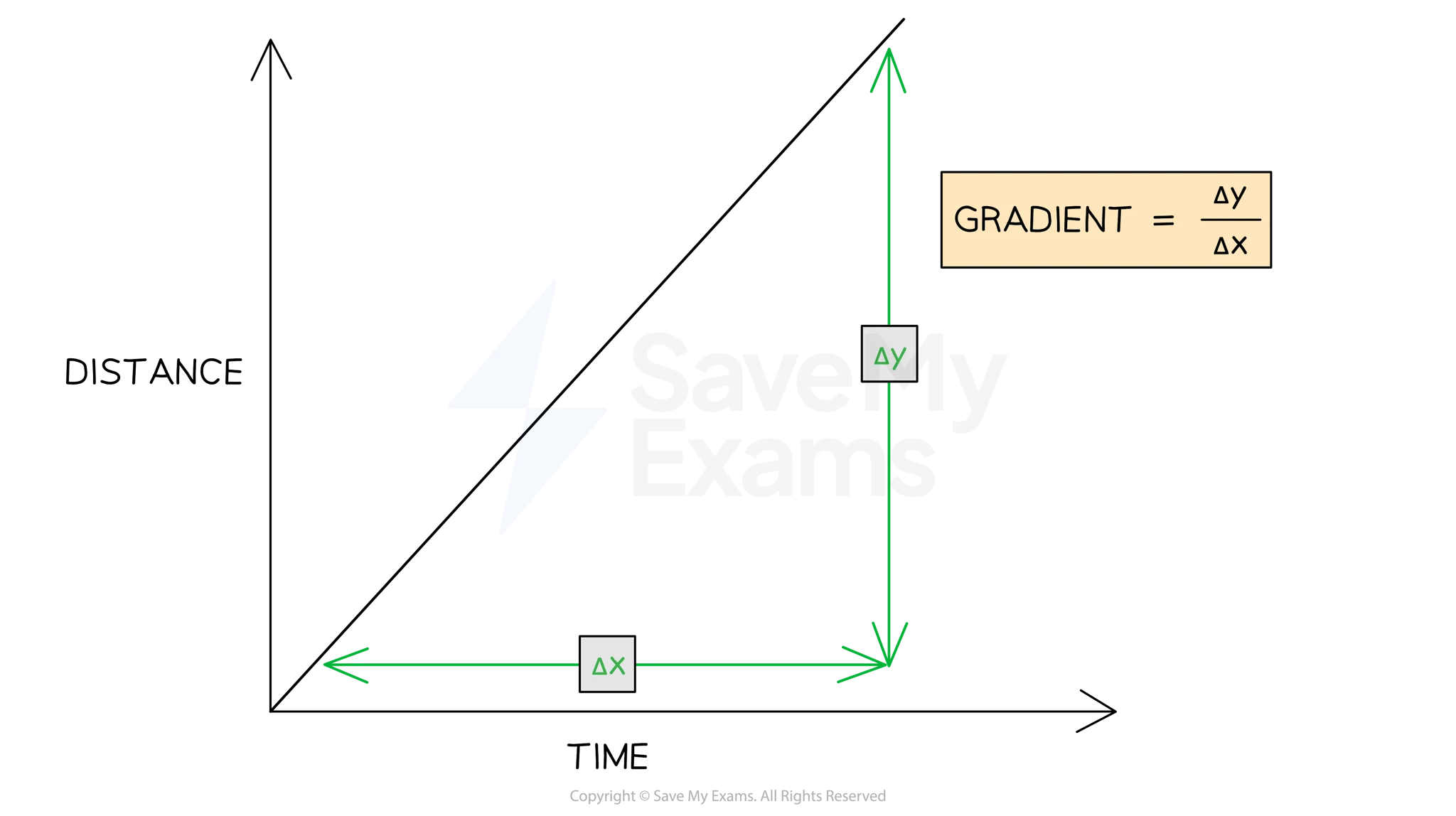
A distance-time graph plots time on the horizontal axis and distance on the vertical axis. The gradient represents speed at any instant:
- A horizontal line indicates the object is at rest (gradient = 0).
- A straight line with constant gradient indicates motion at constant speed.
- A curve with increasing gradient indicates acceleration, as speed increases over time.
- A curve with decreasing gradient indicates deceleration, as speed decreases over time.
Worked example: Speed calculation from the graph requires dividing the rise by the run between two points on the line.
For example, if an object moves from position 0 m at time 0 s to 12 m at time 4 s, the speed is $\frac{12 - 0}{4 - 0} = 3\text{ m/s}$.
Speed-Time Graphs
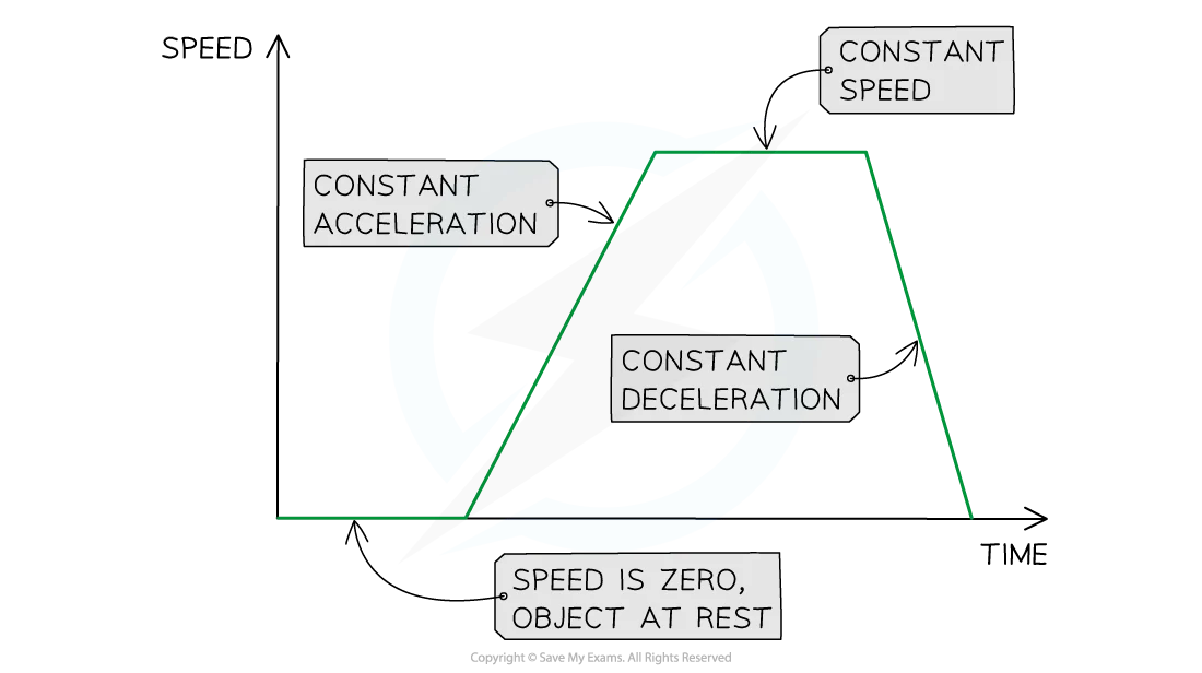
A speed-time graph plots time on the horizontal axis and speed on the vertical axis. Key interpretations include:
- A line on the time axis indicates zero speed (object at rest).
- A horizontal line indicates constant speed.
- A straight line from the origin indicates constant acceleration, with speed increasing linearly.
- A curved line indicates changing acceleration.
The area under the speed-time graph calculates total distance traveled.
For constant speed, distance equals the rectangular area (speed × time).
For constant acceleration, distance equals the triangular area ($\frac{1}{2} \times \text{base} \times \text{height}$).
Deceleration produces negative acceleration, represented by a negative gradient on the graph.
Worked example: An object starts from rest and accelerates to 10 m/s in 5 seconds.
The acceleration is $a = \frac{10 - 0}{5 - 0} = 2\text{ m/s}^2$. Distance covered equals the triangular area: $\frac{1}{2} \times 5 \times 10 = 25\text{ m}$.
Acceleration
Acceleration measures velocity change over time:
$$a = \frac{\Delta v}{t} = \frac{u - v}{t}$$
Free fall describes motion under gravity alone. Near Earth’s surface, gravitational acceleration approaches $g \approx 9.8\text{ m/s}^2$ downward. In uniform gravitational fields without resistance, objects experience constant downward acceleration.
Calculating total distance based on initial velocity
$$ a= \frac{u - v}{t} $$
Where $u$ = initial velocity and $v$ = final velocity
Rearranging this formula we get (equation 1): $$v = u + at$$
Average velocity ($v_{\text{avg}}$) is calculated as (equation 2): $$v_{\text{avg}} = \frac{u + v}{2}$$
Combining with equation 1 and 2: $$v_{\text{avg}} = \frac{u + (u + at)}{2}$$ $$v_{\text{avg}} = \frac{2u + at)}{2}$$ Equation 3: $$v_{\text{avg}} = u + \frac{1}{2}at$$ Distance calculation: $$s = v_\text{avg}\times t$$ $$s = (u + \frac{1}{2}at) \times t$$ $$s = ut + \frac{1}{2}at^2$$
Worked example: An object falls 10 meters from rest.
Using $s = ut + \frac{1}{2}at^2$ with $u = 0$, $a = 9.8\text{ m/s}^2$, and $s = 10\text{ m}$:
$10 = \frac{1}{2}(9.8)t^2$,
giving $t^2 = 2.04$, so $t = 1.43\text{ s}$.
Terminal Velocity
In real conditions, air or liquid resistance opposes gravitational force.
- As an object falls faster, resistance increases until it equals the downward force of gravity.
- At this equilibrium, acceleration becomes zero and the object moves at terminal velocity.
- Terminal velocity depends on object mass, shape, surface area, and fluid density.
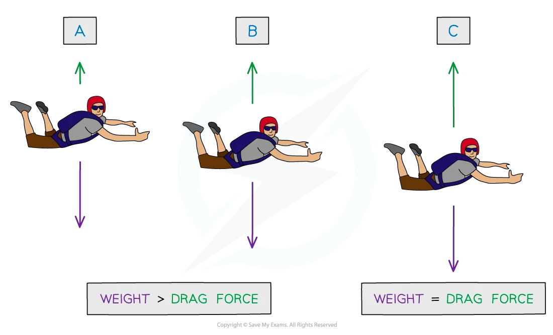
Worked example: A skydiver reaches terminal velocity when drag force equals weight.
If mass is 70 kg and terminal speed is 55 m/s, gravity provides $mg = 70 \times 9.8 = 686\text{ N}$
The drag force at terminal velocity equals this value, preventing further acceleration.